Exploring Passenger Survival in a Plane Crash 
Team:
- 1705012 Akarsh Srivastava
- 1705019 Aniket Das
- 1705068 Sanat B. Singh
- 1705689 Biswajeet Sahoo
This notebook covers the Machine Learning process used to analyse the plane crash survivors data provided in Classification_train.csv and Classification_test.csv
The method used for predictions is Logistic Regression which gives us an accuracy of 95%
Importing Necessary Libraries
import numpy as np
import seaborn as sns
import pandas as pd
import matplotlib.pyplot as plt
Importing warnings module to ignore FutureWarning and DeprecatedWarning
These warnings show us what features might get deprecated in future versions. The features work fine on the latest version as of today 3rd Nov 2018
import warnings
warnings.filterwarnings("ignore", category=FutureWarning)
warnings.filterwarnings("ignore", category=DeprecationWarning)
Converting CSV into a DataFrame
A CSV file can be loaded as a DataFrame using pandas.read_csv
After loading, printing info and head to see what we're working with
Information about the features
- PassengerId ID of the passenger
- Survived Passenger survived or not. 1 for Survived, 0 for did not
- Pclass Classes like Business, Economy, etc.
- Name
- Sex
- Age
- SibSp Number of Siblings or Spouses
- Parch Number of Parents or Children
- Ticket Ticket Number
- Fare Ticket Fare
- Cabin Cabin Number
- Embarked Embarked from which Airport
dataset=pd.read_csv("Classification_train.csv")
dataset.head()
dataset.info()
Visualising Data
Visualising Data is essential to see which features are more important and which features can be dropped
sns.barplot(x="Embarked", y="Survived", hue="Sex", data=dataset);

As we can see from the above barplot, more females survived in a plane crash by a high margin
sns.heatmap(dataset.corr(), annot=True)

The correlation heatmap shows that Survived is most strongly related to Fare, which means that higher fares mean better security in case of a mishap
Further Analysing the Data
dataset.describe()
We can see that the above description did not account for the columns Name, Sex, Ticket, Cabin, and Embarked as they are non-numeric
Non Numeric Values
The following code gives the number of non-numeric string/categorical data, unique values, and the most frequent values with their frequency
dataset.describe(include=['O'])
dataset.head()
There seem to be some NaN values in the column Cabin
This shows that no data was availabe for the particular value.
Getting NaN values is common when dealing with real-world data and other columns might have missing data as well. We should check for these gaps before trying to apply any Machine Learning algorithms to the dataset.
Non-Existent Data
Thankfully, a DataFrame class contains a function isnull() which checks for NaN values and returns a boolean value True or False.
We can count the number of NaN using sum() method
dataset.isnull().sum()
dataset[['Pclass','Survived']].groupby(by=['Pclass'],as_index=False).mean() # p1 class passenger survived more
Removing Unimportant Data
By analysing at the dataset we see that the following features play an insignificant role in survivability.
- PassengerId Irrelevant to survival
- Name The title(Dr. Mr. etc) may or may not be useful high chance of irrelevance
- Cabin Too many
NaN/nullvalues might interfere with the accuracy - Ticket Fare has already been considered thus eliminating the need to analyse the ticket number
Cleaning the Dataset
We can drop the unimportant columns from the dataset
Printing the head() to see what we're left with
dataset = dataset.drop(columns=['PassengerId', 'Name', 'Ticket', 'Cabin'])

dataset.head()
Resolving NaN values
The Embarked column is a non-numeric categorical set with only one missing element.
The following code fills the NaN value with the most frequent value
# Getting the most occured element using pandas get_dummies()
most_occ = pd.get_dummies(dataset['Embarked']).sum().sort_values(ascending=False).index[0]
# The above snippet makes a descending sorted array of the Embarked column and gets the first value

def replace_nan(x):
#Function to get the most occured element in case of null else returns the passed value
    if pd.isnull(x):
        return most_occ
    else:
        return x

#Mapping the dataset according to replace_nan() function
dataset['Embarked'] = dataset['Embarked'].map(replace_nan)
Splitting into Features and Dependent Variables
X will contain all the features
y will contain all the values observed that is the Survived column
So far, we've been dealing with the training set
# Select all rows and all columns except 0
X=dataset.iloc[:,1:8].values

# Select all rows from column 0
y=dataset.iloc[:,0].values
Importing the Test Data
Since we've dropped unimportant features from our training data, the testing data must also be in the same format for accurately predicting the result. Using the same cleaning process as we did with the train dataset
# Load CSV into DataFrame
X_test=pd.read_csv("Classification_test.csv")
y_test=pd.read_csv("Classification_ytest.csv")
# Load CSV into DataFrame
X_test=pd.read_csv("Classification_test.csv")
y_test=pd.read_csv("Classification_ytest.csv")

X_test.head()
X_test is in the same format as our dataset, excluding the Survived Column
Columns that need to be dropped are :
- PassengerId
- Name
- Ticket
- Cabin
X_test= X_test.drop(columns = ['PassengerId', 'Name', 'Ticket', 'Cabin'], axis=1).iloc[:,:].values
y_test.head()
y_test only needs to drop the PassengerId column
y_test=y_test.drop(columns = 'PassengerId', axis=1).iloc[:,:].values
Now that the train and test data is in the same format, we can proceed to manipulation of data
Using Imputer to fill NaN values
Age column has many NaN values which we will fill with the median/most frequent age from the dataset
Fare column has some NaN values in the test dataset which we plan on filling with the mean fare
# Age column having 177 missing values : dataset['Age'].isnull().sum() in training
# Also for test dataset.

from sklearn.preprocessing import Imputer

# Check for NaN values and set insert strategy to median
imputer = Imputer(missing_values = 'NaN', strategy = 'median', axis = 0)
# imputer only accepts 2D matrices
# Passing values [:, n:n+1] only passes the nth columnn
# Here the 2nd column is the Age
imputer = imputer.fit(X[:,2:3])
X[:,2:3] = imputer.transform(X[:,2:3])

imputer = Imputer(missing_values = 'NaN', strategy = 'median', axis = 0)
imputer = imputer.fit(X_test[:,2:3])
X_test[:,2:3] = imputer.transform(X_test[:,2:3])

# Using insert strategy mean
imputer = Imputer(missing_values = 'NaN', strategy = 'mean', axis = 0)
# The 5th column is the Fare
imputer = imputer.fit(X_test[:,5:6])
X_test[:,5:6] = imputer.transform(X_test[:,5:6])
After the above snippet has executed, imputer will have replaced all the NaN values with the specified insert strategy.
Now we can move on to encoding and fitting the dataset into an Algorithm
Encoding
Label Encoding
LabelEncoder is used to convert non-numerical string/categorical values into numerical values which can be processed using various sklearn classes
It encodes values between 0 and n-1; where n is the number of categories
The features which need encoding are:
- Sex
- Embarked
from sklearn.preprocessing import LabelEncoder, OneHotEncoder
labelencoder_X = LabelEncoder()

# Column 6 is Embarked
X[:, 6] = labelencoder_X.fit_transform(X[:, 6])
X_test[:, 6] = labelencoder_X.fit_transform(X_test[:, 6])

# Column 1 is Sex
X[:, 1] = labelencoder_X.fit_transform(X[:, 1])
X_test[:, 1] = labelencoder_X.fit_transform(X_test[:, 1])
One Hot Encoding
Often when we use LabelEncoder on more than 2 categories the Machine Learning algorithm might try to find a relation between the values such as Increasing or Decreasing or in a pattern. This results in lower accuracy.
To avoid this we can further encode the Labels using OneHotEncoder, it takes a column which has categorical data, which has been label encoded, and then splits the column into multiple columns. The numbers are replaced by 1s and 0s, depending on which column has what value. Thus the name OneHotEncoder
onehotencoder = OneHotEncoder(categorical_features = [0,1,6])
# 0 : Pclass column
# 1 : Sex
# 6 : Embarked

# OneHotEncoder takes and array as input
X = onehotencoder.fit_transform(X).toarray()
X_test = onehotencoder.fit_transform(X_test).toarray()
With One Hot Encoding complete, we can proceed to fit the data into our LogisticRegressor
Predicting the Output
LogisticRegression
LogisticRegression is used only when the dependent variable/prediction is binary i.e only consists of two values. LogisticRegression is used to describe data and to explain the relationship between one dependent binary variable and one or more nominal, ordinal, interval or ratio-level independent variables.
from sklearn.linear_model import LogisticRegression

#Initializing the regressor
lr = LogisticRegression()

# Fitting the regressor with training data
lr.fit(X,y)

# Getting predictions by feeding features from the test data
y_pred = lr.predict(X_test)
Checking the Predictions
Creating a scatter plot of actual versus predicted values
plt.scatter(y_test, y_pred, marker='x')

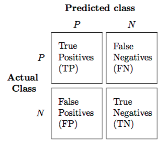
Confusion Matrix
ConfusionMatrix is used to compare the data predicted versus the actual output.
It is a matrix in the form:
from sklearn.metrics import confusion_matrix

cm = confusion_matrix(y_test,y_pred)
print(cm)
Classification Report
To get the accuracy, we use ClassificationReport which measures the acuracy of the algorithm based on a ConfusionMatrix
An ideal classifier with 100% accuracy would produce a pure diagonal matrix which would have all the points predicted in their correct class.
from sklearn.metrics import classification_report

print(classification_report(y_test, y_pred))
Conclusion
After analysing the given dataset and using LogisticRegression on the features, we see that the algorithm can accurately predict the survivability of a Passenger 95% of the time.